Method
The rendering speed of 3D Gaussian Splatting (3D-GS) is primarily determined by two factors:
- The number of Gaussians allocated to each pixel, and
- The total number of Gaussians in the scene.
Speedy-Splat introduces methods to address each of these.
Number of Gaussians Allocated to Each Pixel
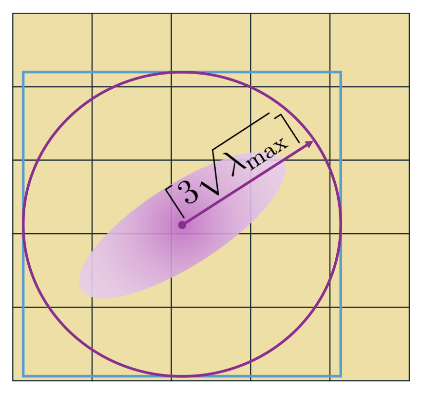
Gaussian splatting is a tile-based renderer that assigns Gaussians to tiles of pixels by calculating their intersections. As shown in Figure 1a, the current algorithm for computing Gaussian-to-tile intersections is overly conservative in estimating the tile extent of Gaussians. We propose two algorithms to increase rendering speed by making exact localizations: SnugBox and AccuTile.


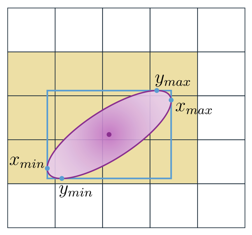
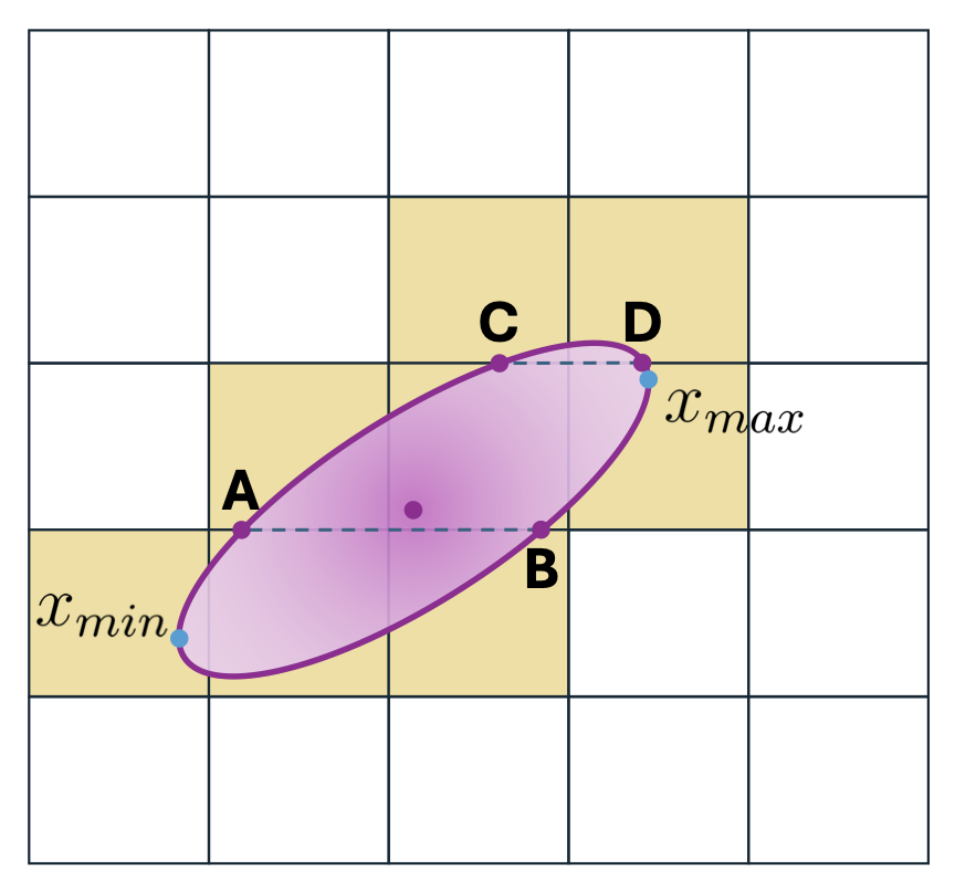
Figure 1: Gaussian tile allocation by method. (a) 3D Gaussian Splatting overestimates the Gaussian-to-tile intersections by relying solely on the maximum eigenvalue \(\lambda_{\max}\) of the projected 2D covariance for its computation. (b) Our SnugBox method finds the axis-aligned tight bounding box of the Gaussian and corresponding rectangular tile extent in constant time. (c) Our AccuTile method extends SnugBox to quickly compute exact Gaussian-to-tile intersections.
SnugBox
A threshold on \( \alpha_i(p) = \sigma_i g_i(p) \), where \( \sigma_i \) is the opacity of Gaussian \( \mathcal{G}_i \) and \( g_i(p) \) is its value at pixel \( p \) when it is projected to the image plane, determines the exact pixel exent of \(\mathcal{G}_i \) as an ellipse. We compute a tight bounding box — the SnugBox presented in Figure 1b — around this ellipse by calculating the four points where its first derivative is zero. After dividing these points by tile size, rounding, and clipping to the image boundary, we obtain the rectangular tile extent of \(\mathcal{G}_i \) in constant time.
AccuTile
Extending our SnugBox algorithm, we compute the exact tile intersection of Gaussian \(\mathcal{G}_i \) by iterating over the shorter side of the SnugBox tile extent. In each row or column, we identify the exact tile extent by finding the minimum and maximum points of the ellipse inside it — all tiles between these points intersect the ellipse. The insight of our AccuTile algorithm, illustrated in Figure 1c and detailed below, is that these exact Gaussian-to-tile intersections can be computed efficiently such that only two points need to be computed per row or column of the SnugBox.
Total Number of Gaussians
Recent post-hoc pruning technique PUP 3D-GS [1] finds that approximately 90% of Gaussians can be pruned from pretrained scenes while retaining high visual fidelity. Our efficient pruning score identifies a reparameterization of their sensitivity pruning score that improves its memory efficiency by 36×, allowing us to integrate it into the 3D-GS training pipeline via two distinct modalities: Soft Pruning and Hard Pruning.
Efficient Pruning Score
PUP 3D-GS [1] computes a sensitivity pruning score \( U_i \) for each Gaussian \( \mathcal{G}_i \) as the log determinant of the second order approximation of the \( L_2 \) reconstruction error with respect to its mean and scaling parameters \( \mu_i \) and \( s_i \) :
\[ U_i = \log \left| \nabla_{\mu_i,s_i}^2 L_2 \right| = \log \left| \sum_{\phi \in \mathcal{P}_{gt}} \nabla_{\mu_i,s_i} I_{\mathcal{G}}(\phi) \nabla_{\mu_i,s_i} I_{\mathcal{G}}(\phi)^T \right|, \] \[ \begin{aligned} U_i &= \log \left| \nabla_{\mu_i,s_i}^2 L_2 \right| \\ &= \log \left|\sum_{\phi\in \mathcal{P}_{gt}} \nabla_{\mu_i,s_i} I_{\mathcal{G}}(\phi)\nabla_{\mu_i,s_i} I_{\mathcal{G}}(\phi)^T \right|, \end{aligned} \]
where \( \mathcal{P}_{gt} \) is the set of all training camera poses and \( I_{\mathcal{G}}(\phi) \) is the rendered view for pose \( \phi \). This second order approximation is shown to be exact when the \(L_1\) error over \( \mathcal{P}_{gt} \) is zero.
We update this score by computing it with respect to the projected Gaussian values \( g_i \) instead:
\[ \tilde{U}_i = \log \left| \sum_{\phi \in \mathcal{P}_{gt}} \nabla_{g_i} I_{\mathcal{G}}(\phi) \nabla_{g_i} I_{\mathcal{G}}(\phi)^T\right|. \]
Because \( g_i \) is a scalar at each pixel and \( \log \) is monotonically increasing, we can simplify the score to:
\[ \tilde{U}_i = \sum_{\phi \in \mathcal{P}_{gt}} \nabla_{g_i} I_{\mathcal{G}}(\phi)^2. \]Our efficient pruning score reduces the storage requirement of the sensitivity pruning score by 36× and allows us to integrate it into the 3D-GS training pipeline.
Soft Pruning and Hard Pruning
We empirically observe that the \( L_1 \) loss converges quickly during training and deploy our efficient pruning score via two modalities:
- Soft Pruning, performed during the densification stage, and
- Hard Pruning, performed after the densification stage.
Together, they reduce the number of Gaussians in the model by approximately 90%, increasing rendering and training speed while maintaining image quality.
Results
The AccuTile Algorithm
To match the example in Figure 1c, the algorithm outlined below is applied to the rows of the SnugBox tile extent bounding box. In practice, it is applied along the smaller side of the tile extent. The subscripts \(t\), \(b\), \(l\), and \(r\) represent the top, bottom, left, and right sides, respectively.
\[ \textbf{Input:} \] \[ \begin{aligned} &\text{Gaussian Ellipse Boundary } \class{highlight-purple}{\mathbf{E}} \\ &\text{SnugBox Bounding Box } \class{highlight-blue}{\mathbf{B}} \\ &\text{SnugBox Tile Extent Rectangle } \class{highlight-yellow}{\mathbf{R}} \end{aligned} \] \[ \textbf{Procedure:} \] \[ \begin{aligned} &\text{Tile count } \class{highlight-yellow}{\mathbf{C}} \gets 0 \\ &\class{highlight-yellow}{\text{line}_{\min}} \gets \class{highlight-yellow}{\mathbf{R}_b} \\ &\textbf{if } \class{highlight-yellow}{\text{line}_{\min}} \geq \class{highlight-blue}{\mathbf{B}_b} \textbf{ then } \\ &\quad \class{highlight-purple}{\mathbf{i}_{\min}} \gets \text{Intersections}( \class{highlight-yellow}{\text{line}_{\min}}, \class{highlight-purple}{\mathbf{E}}) \\ &\textbf{for row } \class{highlight-yellow}{r} \textbf{ in } \class{highlight-yellow}{\mathbf{R}} \textbf{ do } \\ &\quad \class{highlight-yellow}{\text{line}_{\max}} \gets \class{highlight-yellow}{r_t} \\ &\quad \textbf{if } \class{highlight-yellow}{\text{line}_{\max}} \leq \class{highlight-blue}{\mathbf{B}_t} \textbf{ then } \\ &\quad \quad \class{highlight-purple}{\mathbf{i}_{\max}} \gets \text{Intersections}( \class{highlight-yellow}{\text{line}_{\max}}, \class{highlight-purple}{\mathbf{E}}) \\ &\quad \class{highlight-purple}{e_{\min}} \gets \begin{cases} \class{highlight-blue}{\mathbf{B}_l} & \text{if } \class{highlight-blue}{\mathbf{B}_l} \text{ in }\class{highlight-yellow}{r} \\ \min(\class{highlight-purple}{\mathbf{i}_{\min}}, \class{highlight-purple}{\mathbf{i}_{\max}}) & \text{otherwise} \end{cases} \\ &\quad \class{highlight-purple}{e_{\max}} \gets \begin{cases} \class{highlight-blue}{\mathbf{B}_r} & \text{if } \class{highlight-blue}{\mathbf{B}_r} \text{ in }\class{highlight-yellow}{r} \\ \max(\class{highlight-purple}{\mathbf{i}_{\min}}, \class{highlight-purple}{\mathbf{i}_{\max}}) & \text{otherwise} \end{cases} \\ &\quad \class{highlight-yellow}{\text{tile}_{\min}}, \class{highlight-yellow}{\text{tile}_{\max}} \gets \text{Convert}(\class{highlight-purple}{e_{\min}}, \class{highlight-purple}{e_{\max}}) \\ &\quad \class{highlight-yellow}{\mathbf{C}} \gets \class{highlight-yellow}{\mathbf{C}} + (\class{highlight-yellow}{\text{tile}_{\max}} - \class{highlight-yellow}{\text{tile}_{\min}}) \\ &\quad \text{Process}(\class{highlight-yellow}{\text{tile}_{\min}}, \class{highlight-yellow}{\text{tile}_{\max}}) \\ &\quad \class{highlight-purple}{\mathbf{i}_{\min}} \gets \class{highlight-purple}{\mathbf{i}_{\max}} \\ &\textbf{return } \class{highlight-yellow}{\mathbf{C}} \end{aligned} \]
The following walkthrough outlines each step of the example illustrated in Figure 1c, where the AccuTile algorithm processes the SnugBox output from Figure 1b to find the exact tile extent:
The tile extent rows from Snugbox, shown in Figure 1b, are processed starting from the bottom. The lower tile row boundary falls below the bounding box, so no initial intersection is computed. The upper boundary lies below the top of the bounding box, so intersection points \(A\) and \(B\) are calculated. \(x_{\min}\) is assigned as this row's minimum ellipse extent \(e_{\min}\) because it lies within the row, and \(B\) is assigned as its maximum ellipse extent \(e_{\max}\) because it is the maximal point. Consequently, this row's tile extent is from the tile containing \(x_{\min}\) to the tile containing \(B\). For the next row, we keep points \(A\) and \(B\) and compute upper boundary points \(C\) and \(D\). \(A\) and \(x_{\max}\) are assigned as the row's \(e_{\min}\) and \(e_{\max}\), and the tiles containing them are its tile extent. Finally, for the last row, \(C\) and \(D\) are kept; no additional points are computed because the row's upper boundary is above the bounding box. Thus, the tile extent of this row is the tiles containing \(C\) and \(D\).
BibTeX
@InProceedings{HansonSpeedy,
    author    = {Hanson, Alex and Tu, Allen and Lin, Geng and Singla, Vasu and Zwicker, Matthias and Goldstein, Tom},
    title     = {Speedy-Splat: Fast 3D Gaussian Splatting with Sparse Pixels and Sparse Primitives},
    booktitle = {Proceedings of the Computer Vision and Pattern Recognition Conference (CVPR)},
    month     = {June},
    year      = {2025},
    pages     = {21537-21546},
    url       = {https://speedysplat.github.io/}
}
Related Work
For additional papers on efficient 3D Gaussian Splatting, see our group’s related work below. If your research builds on ours, we encourage you to cite these papers.
- PUP-3DGS (CVPR 2025) [BibTeX] — Prune 90% of primitives from any pretrained 3D Gaussian Splatting model using a mathematically principled sensitivity score, more than tripling rendering speed while retaining more salient foreground information and higher visual fidelity than previous techniques at a substantially higher compression ratio.
- SpeeDe3DGS (CVPR 2026) [BibTeX] — Boost DeformableGS rendering speed from 20 to 276 FPS using temporal sensitivity pruning and groupwise SE(3) motion distillation, all while preserving the superior image quality of per-Gaussian neural motion.